Linear Regression

Table of Contents show

Regression

A regression model is a mathematical equation that describes the relationship between two or more variables
A simple regression model includes only two variables: one independent and one dependent.
The dependent variable is the one being explained and the independent variable is the one used to explain the variation in the dependent variable

Remember this:

Y=mX+B?

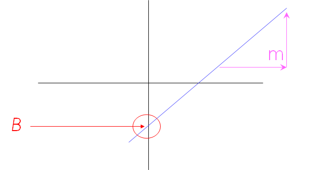
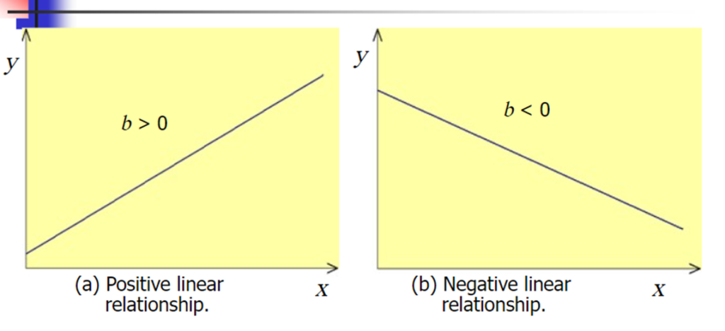
A slope of 2 means that every 1-unit change in X yields a 2-unit change in Y.

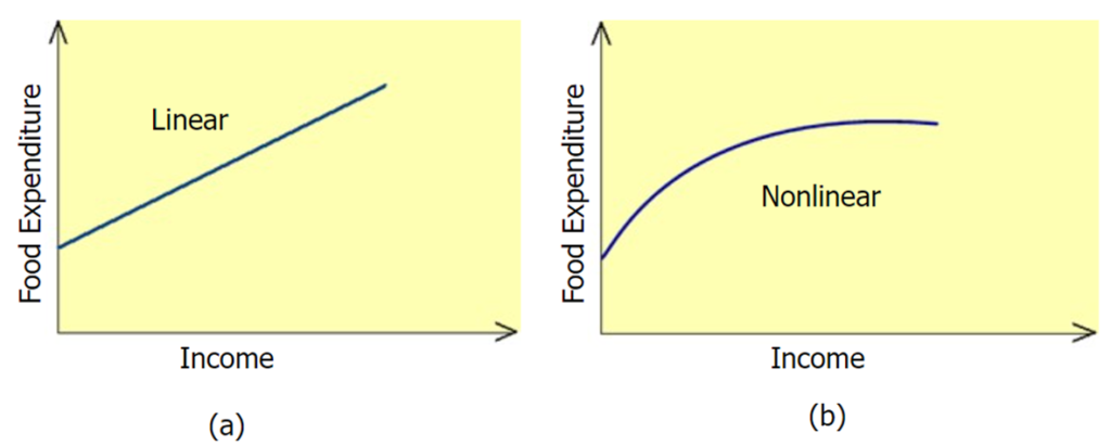
A (simple) regression mode that gives a straight-line relationship between two variables is called a linear regression model

Simple Linear Regression Analysis

Scatter Diagram
Least Square Line
Interpretation of slope and intercept
Assumptions of Regression Analysis

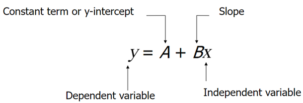
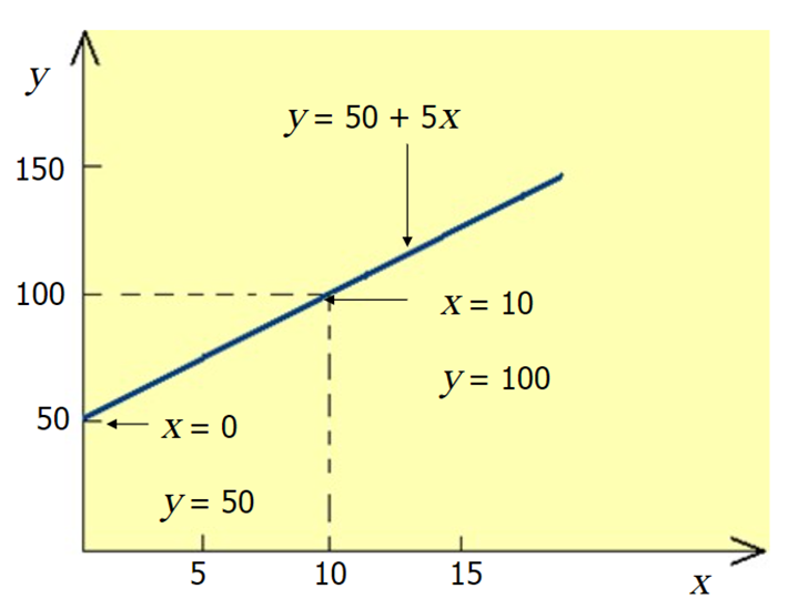
In the regression model, y= A+Bx+C

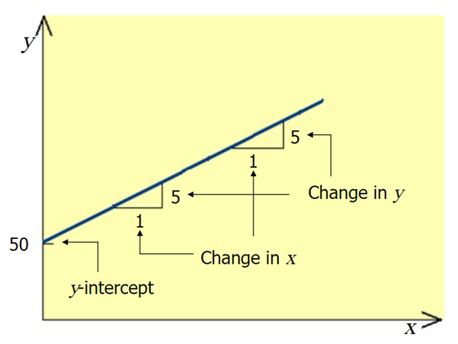
A is called the y-intercept or constant term
B is the slope
C is the random error
The dependent and independent variables are y and x respectively

Sum of Squared Error (SSE)

The sum of Squared error (SSE) is,

\[{SSE} = \sum{e^2} = \sum{(y – ŷ)^2}\]

The values of a and b that gives the minimum SSE are called least square estimates and the regression line obtained with these estimates is called the least square line

The Least Squares line

For the least squares regression line,

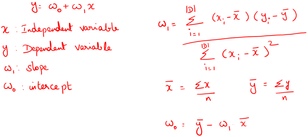
Interpretation of slope and intercept

The value of intercept in the regression model gives the change in y due to change of one unit in x

Assumptions of the Regression Model

Assumption 1: The random error has a mean equal to zero for each x
Assumption 2: The errors associated with different observations are independent
Assumption 3: For any given x, the distribution of error is normal
Assumption 4: The distribution of population errors for each x has the same (constant) standard deviation

Degrees of Freedom

The degrees of freedom for a simple linear regression model are,

df = n-2

Standard deviation of errors is calculated as

\[S_e = \sqrt{{{SS}_{yy} – {bSS}_{xy}}\over {n-2}}\]

Where,

\[SS_{yy} = \sum{y^2} – {{(\sum y)^2}\over {n}}\]

Total Sum of Squares (SST)

The total sum of squares, denoted by SST, is calculated as,

\[SST = \sum{y^2} – {{(\sum y)^2}\over {n}}\]

Regression Sum of Squares (SSR)

The regression sum of squares denoted by SSR is,

\[SSR = SST – SSE\]

Coefficient of determination

The Coefficient of determination denoted by r² , represents the proportion of SST that is explained by the use of the regression model. The computational formula for r² is,

\[r^2 = {{bSS}_{xy} \over {SS}_{yy}}\]

and

\[0 \le r^2 \le 1\]

The higher the value of r², the more successful is simple linear regression model in explaining y variation

Multiple Linear Regression

Multiple linear regression: involves more than one predictor variable

Training data is of the form (X₁, y₁), (X₂, y₂),…, (X_|D|, y_|D|)
Ex. For 2-D data, we may have: y = w₀ + w₁ x₁+ w₂ x₂

Advanced Python

Linear Regression

Regression

Remember this: