Logistic Regression
- Linear Regression is used to model continuous valued functions
- Can it also be used to predict categorical labels?
- Logistic Regression: The probability of some event occurring as a linear function of a set of predictor variables

- Suppose the numerical values of 0 and 1 are assigned to the two outcomes of a binary variable
- Often the 0 represents a negative response and 1 represents a positive response
- The mean of this variable will be the proportion of the positive responses
- If p is the proportion of observation with an outcome of 1, then 1-p is the probability of a outcome of 0
- odds: the ratio p/1-p
- Odds ratio: the probability of winning over losing
- logit is the logarithm of the odds or just log odds Mathematically, the logit transformation is written as
l=logit(p) = ln(p/1-p)Support Vector Machine
- A relatively new classification method for both linear and nonlinear data
- It uses a nonlinear mapping to transform the original training data into a higher dimension
- With the new dimension, it searches for the linear optimal separating hyperplane (i.e., “decision boundary”)
- With an appropriate nonlinear mapping to a sufficiently high dimension, data from two classes can always be separated by a hyperplane
- SVM finds this hyperplane using support vectors (“essential” training tuples) and margins (defined by the support vectors)
SVM-History and Applications
- Vapnik and colleagues (1992)—groundwork from Vapnik & Chervonenkis’ statistical learning theory in 1960s
- Features: training can be slow but accuracy is high owing to their ability to model complex nonlinear decision boundaries (margin maximization)
- Used for: classification and numeric prediction
- Applications: handwritten digit recognition, object recognition, speaker identification, benchmarking time-series prediction tests
SVM—General Philosophy
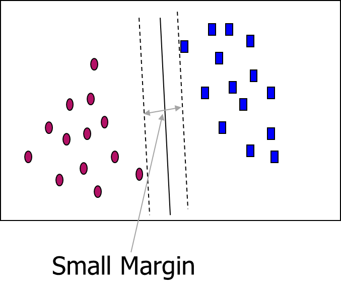
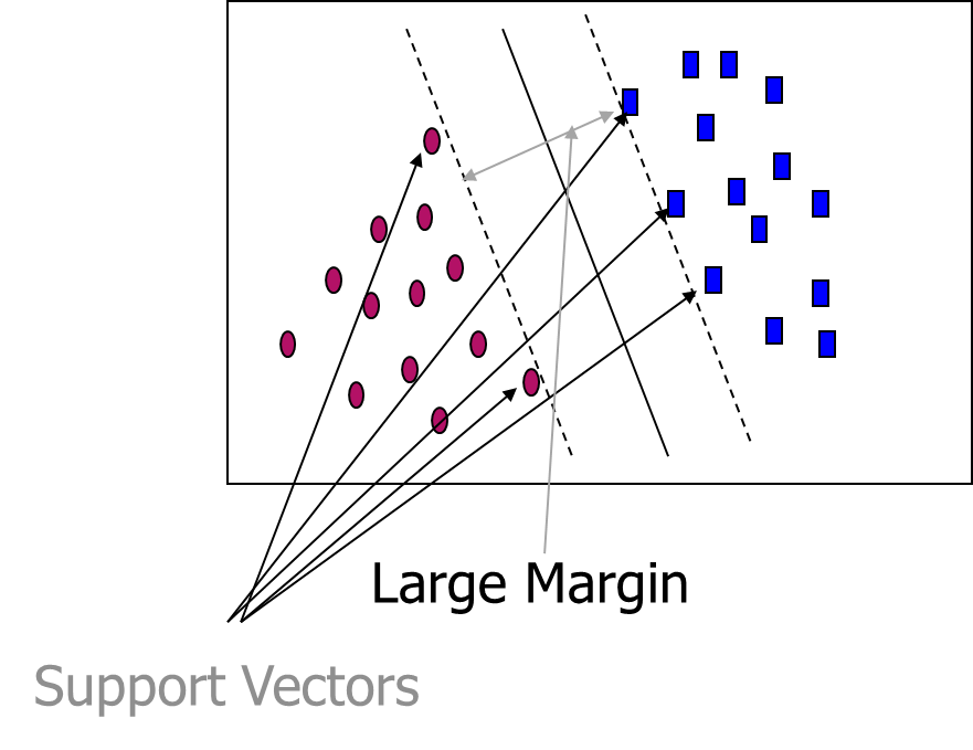
SVM—Margins and Support Vectors
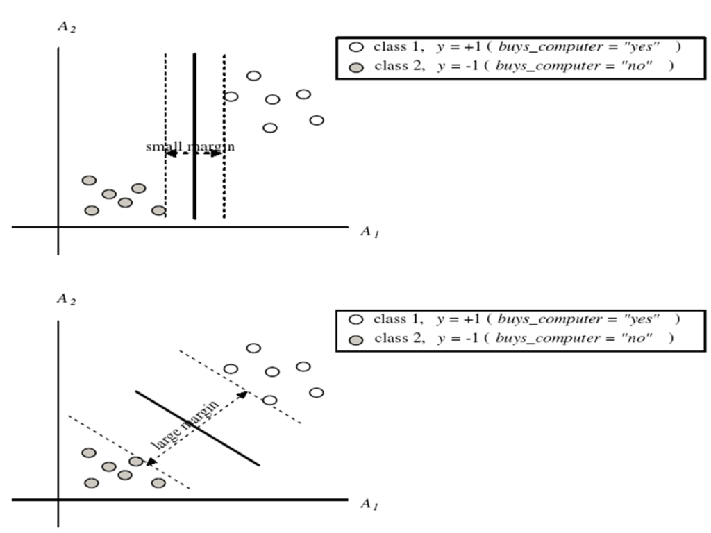
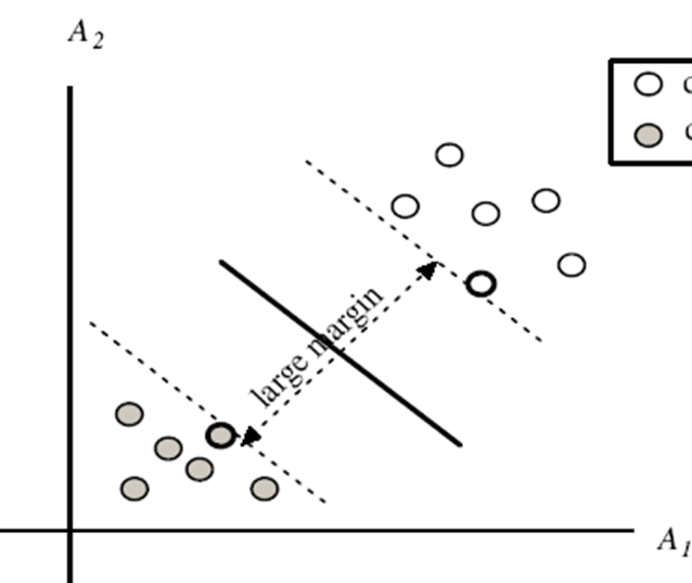
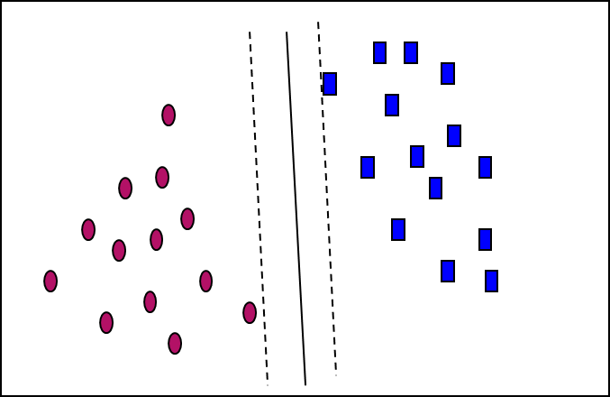
SVM—When Data Is Linearly Separable
- Let data D be (X1, y1), …, (X|D|, y|D|), where Xi is the set of training tuples associated with the class labels yi
- There are infinite lines (hyperplanes) separating the two classes but we want to find the best one (the one that minimizes classification error on unseen data)
- SVM searches for the hyperplane with the largest margin, i.e., maximum marginal hyperplane (MMH)

SVM—Linearly Separable
- A separating hyperplane can be written as
- W ● X + b = 0
- where W={w1, w2, …, wn} is a weight vector and b a scalar (bias)
- For 2-D it can be written as
- w0 + w1 x1 + w2 x2 = 0
- The hyperplane defining the sides of the margin:
- H1: w0 + w1 x1 + w2 x2 ≥ 1 for yi = +1, and
- H2: w0 + w1 x1 + w2 x2 ≤ – 1 for yi = –1
- Any training tuples that fall on hyperplanes H1 or H2 (i.e., the
sides defining the margin) are support vectors - This becomes a constrained (convex) quadratic optimization problem: Quadratic objective function and linear constraints à Quadratic Programming (QP) à Lagrangian multipliers
Why Is SVM Effective on High Dimensional Data?
The complexity of trained classifier is characterized by the # of support vectors rather than the dimensionality of the data
SVM: Different Kernel functions
Instead of computing the dot product on the transformed data, it is math. equivalent to applying a kernel function K(Xi, Xj) to the original data, i.e., K(Xi, Xj) = Φ(Xi) Φ(Xj)
Typical Kernel Functions

SVM can also be used for classifying multiple (> 2) classes and for regression analysis (with additional parameters)
Working with Iris Dataset
Refer Jupyter notebook for Implementation – To be discussed with Module 5
Accuracy Prediction
Accuracy Measures
Accuracy:
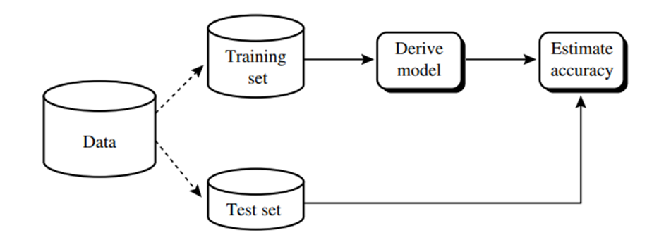
- The accuracy of a classifier on a given test set is the percentage of test set tuples that are correctly classified by the classifier
- Also known as Recognition rate
Error Rate or Misclassification Rate)
- Represented as 1-Acc(M)
- Where Acc(M) is the accuracy of classifier M\
Confusion Matrix
Given m classes, a confusion matrix is a table of at least size m by b
| Predicted (0) | Predicted (1) | |
| Actual (0) | True Negative (TN) | False Positive (FP) |
| Actual (1) | False Negative (FN) | True Positive (TP) |
- N = number of observations
- Accuracy = (TN + TP) / N
- Accuracy = (TN + TP) / (TN+FP+FN+TP)
- Sensitivity = TP / (TP + FN)
- Specificity = TN / (TN + FP)
- Overall error rate = (FP + FN) / N
- False Negative Error Rate = FN / (TP+FN)
- False Positive Error Rate = FP / (TN+FP)
- Precision = TP / TP + FP
- Recall = TP / TP + FN
- F1 Score =(2 *precision *recall) / (precision + recall)
| Predicted (0) | Predicted (1) | |
| Actual (0) | True Negative (TN) | False Positive (FP) |
| Actual (1) | False Negative (FN) | True Positive (TP) |
Alternate Accuracy Measures
Predicted Class
| Actual Class | C0 | C1 |
| C0 | N0,0 = number of C0 cases classified correctly | N0,1 = number of C0 clases classified incorrectly as C0 |
| C1 | N1,0 = number of C1 cases classified incorrectly as C0 | N1,1 = number of C1 cases classified correctly |
If “C1” is important class
- Sensitivity = % of “C1” class correctly classified
- Sensitivity = N1,1 / (N1,0 + N1,1)
- Specificity = % of “C0” class correctly classified
- Specificity = N0,0 / (N0,0 + N0,1)
- False Positive rate = % of predicted “C1’s” that were not “C1’s”
- False Negative rate = % of predicted “C1’s” that were not “C1’s”
a
True Negative Rate is known as Specificity
ROC Curves
- ROC – Receiver Operating Characteristic
- Can be used to compare tests / Procedures
- ROC Curves: Simplest case
- Consider diagnostic test for a disease
- Test has 2 possible outcomes:
- Positive = suggesting presence of disease
- Negative
- An individual can test either positive or negative for the disease
ROC Analysis
- True Positives = Test states you have the disease when you do have the disease
- True Negatives = Test states you do not have the disease when you do not have the disease
- False Positives = Test states you have the disease when you do not have the disease
- False Negatives = Test states you have the disease when model says you do not have the disease
Receiver Operating Characteristic
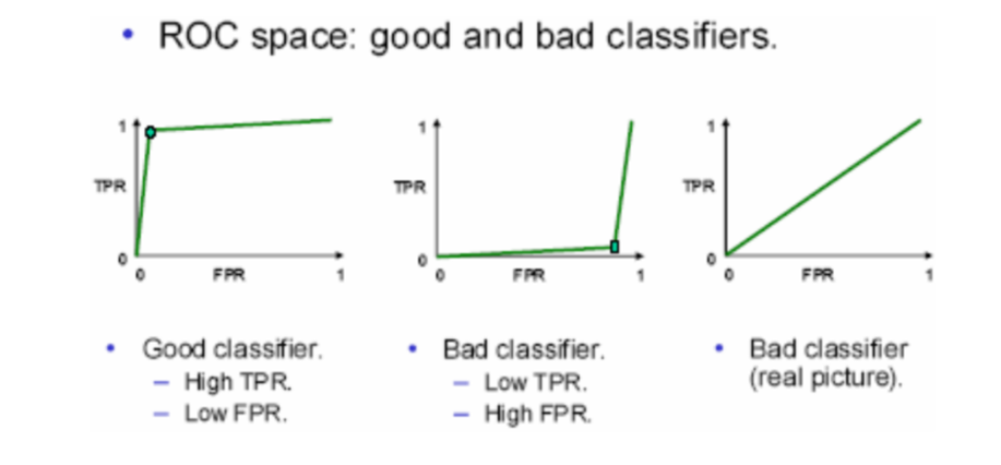
Receiver Operator Characteristic
- True Positive Rate (Sensitivity) on y-axis
- Proportion of positive
- False Positive Rate (Specificity) on x-axis
- Proportion of negative labelled as positive
Predictor Error Measures
Loss functions measure the error between yi and the predicted value (ýi)
Evaluating the accuracy of a classifier or Predictor
Views: 1